[Paper Summary] Complete Parameter Inference for GW150914 Using Deep Learning

---

---

One-sentence Summary

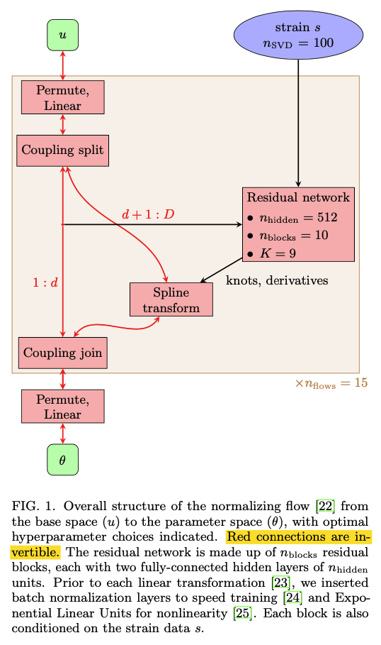
The paper describes a neural network architecture, based on normalizing flows alone, that is able to generate posteriors on the full $D = 15$ dimensional parameter space of quasi-circular binary inspirals, using input data surrounding the first observed GW event, GW150914, from multiple gravitational-wave detectors.

---

Code

• For both 2008.03312 and 2002.07656：
  • 👉 https://github.com/stephengreen/lfi-gw/

---

Background

• Inference is extremely computationally expensive.

  • Run times (MCMC & Nested-samping) for single posterior calculations typically take days for BBH systems and weeks for BNS.
  • In the nearly future, event rates reach one per day or even higher.

• Existing pipelines:

  • LALInference
  • Bilby

• An advantage of likelihood-free methods is that waveform generation is done in advance of training and inference, rather than at sampling time as for conventional methods.

---

Model: normalizing flows

Specifically, a neural spline normalizing flow.

• Conor Durkan, Artur Bekasov, Iain Murray, and George Papamakarios, “Neural spline flows,” (2019), arXiv:1906.04032 [stat.ML].
• Conor Durkan, Artur Bekasov, Iain Murray, and George Papamakarios, “Neural spline flows,” https://github.com/bayesiains/nsf (2019).

---

Training

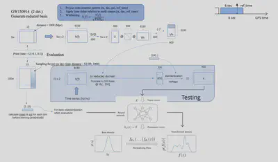
Waveform generation is too costly to perform in real time during training, so we adopt a hybrid approach:

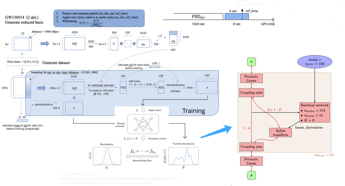
we sample “intrinsic”parameters in advance and save associated waveform polarizations $h^{(i)}_{+,\times}$; at train time we sample “extrinsic” parameters, project onto detectors, and add noise. We used $10^6$ sets of intrinsic parameters, which was sufficient to avoid overfitting.

---

Prior

• The authors consider $\left(m_{i}, \phi_{c}, a_{i}, \theta_{i}, \phi_{12}, \phi_{J L}, \theta_{J N}\right)$ to be intrinsic (10 parameters ($i=1,2$)), so they are sampled in advance of training (see figure):

  • detector-frame masses
    • $m_i \sim U[10,80] \text{ M}_\odot$
  • reference phase
    • $\phi_c\sim U[0,2\pi]$
  • Spin magnitudes
    • $a_i\sim U[0,0.88]$
  • spin angles
    • $\cos(\theta_{i})\sim U[1,-1], \phi_{12}\sim U[0,2\pi], \phi_{J L}\sim U[0,2\pi]$
  • inclination angle
    • $\cos(\theta_{JN})\sim U[-1,1]$

• During the training, they take a uniform prior over the “extrinsic” for sampling:

  • time of coalescence
    • $t_{c,\text{geocent}}\sim U[-0.1,0.1]$
    • (taking $t_{c,\text{geocent}}=0$ to be the GW150914 trigger time)
  • luminosity distance
    • $d_L\sim U(100,1000)\text{ Mpc}$
  • polarization angle
    • $\psi\sim U[0,\pi]$
  • sky position
    • $\alpha\sim U[0,2\pi],\sin(\delta)\sim U[-1,1]$.

• All parameters are rescaled to have zero mean and unit variance before training (see figure).

---

Strain data

• Assuming stationary Gaussian noise
• IMRPhenomPv2 frequency-domain precessing model.
• A frequency range of $[20, 1024]$ Hz
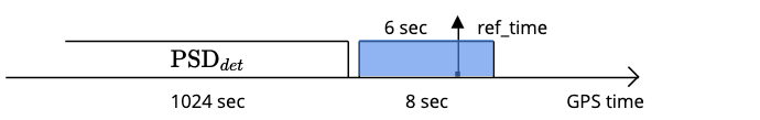
• A waveform duration of 8 s, in which the trigger time at 6th s.
• whiten $h^{(i)}_{+,\times}$ using the noise PSD estimated from 1024 s of detector data prior to the GW150914 event.
• The whitened waveforms are compressed to a reduced-order representation using singular value decomposition. The authors keep the first $n_{SVD}=100$ components during training (see figure).
• The authors pre-prepared a grid of time-translation matrix operators that act on vectors of RB coefficients for relative whitening and time shifting.
• The data is also standardized to have zero mean and unit variance in each component (see figure).

---

Results

• Coding using PyTorch

• 500 epochs

• a batch size of 512

• Initial learning rate: 0.0002 (using cosine annealing)

• Reserved 10% of training set for validation

• Traning took $\sim6$ days with an NVIDIA Quadro P400 GPU

• Testing (see figure) produced samples at a rate of 5,000 per second.

• The authors said that varied $n_{\text{SVD}}$ can be used to imporve the performance.

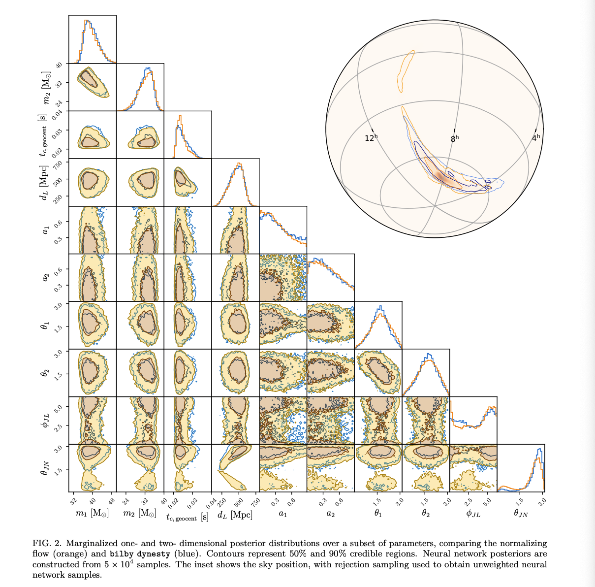
• The authors show their benchmarked result comparing with bilby:
  • Both distributions are clearly in very close agreement.
  • Minor differences in the inclination angle $\theta_{JN}$.
  • FYI: I have reproduced the result and see major differences in the inclination angle.

• The authors claim that their model can be trained to generate any posterior consistent with the prior and the given noise PSD.

  • FYI: I can’t reproduce a evidence to support this claim with other GW events for now.

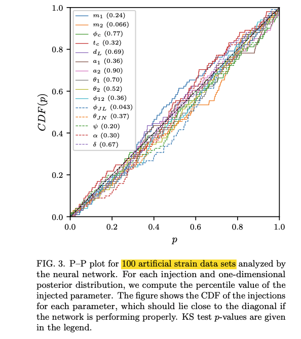
  • A P-P plot is shown to support this claim.

    • My comment: more artificial strain data (>200) and confidence intervals (eg: 95%) around the diagonal are needed.
    • FYI: I have shown 1-$\sigma$ confidence intervals for the P-P plot, and it seems not good enough.

    

---

Remark

1. One approach would be to condition the model on PSD information:

   During training, waveforms would be whitened with respect to a PSD drawn from a distribution representing the variation in detector noise from event to event, and (a summary of) this PSD information would be passed to the network as additional context.

   (PSD samples can be obtained from detector data at random times.)

2. As new and more powerful normalizing flows are developed by computer scientists in the future, they will be straight-forward to deploy to further improve the performance and capabilities of deep learning for gravitational-wave parameter estimation.

---

Appendix for 2002.07656

One slide for all points:

Appendix for 2008.03312

Research notes for the source code. (

Download the PDF )