Lecture 6. Training Neural Networks, part I
Table of Contents
CS231n 课程的官方地址:http://cs231n.stanford.edu/index.html
该笔记根据的视频课程版本是 Spring 2017(BiliBili),PPt 资源版本是 Spring 2018.
另有该 Lecture 6. 扩展讲义资料:
- Neural Nets notes 1 (中译版)
- Neural Nets notes 2 (中译版)
- Neural Nets notes 3 (中译版)
- tips/tricks: [1], [2], [3] (optional)
- [Deep Learning - Nature] (optional)
1. One time setup
这里开始介绍正式训练迭代前,你需要考虑的东西!
1.1 Activation functions
终于开始细讲激活函数了。
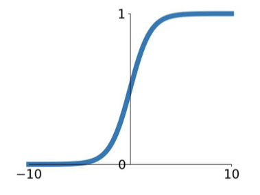
Sigmoid
- Pro
- Squashes numbers to range [0, 1] (有界的)
- Historically popular since they have nice interpretation as a saturating “firing rate” of a neuron
- Con
- Saturated neurons “kill” the gradients(梯度压缩为0)
- Sigmoid outputs are not zero-centered(如果 input 值都同号,会影响当前 neural 也都向同号方向更新参数,这也就是为何要有 zero-mean data)
- exp() is a bit compute expensive
Tanh(x) [LeCun et al., 1991]
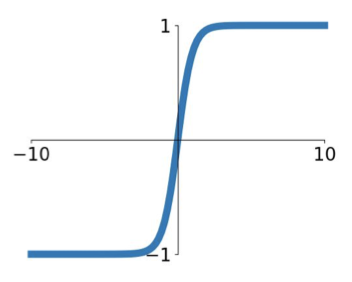
$$ \sigma(x) = \tanh(x) $$
- Pro
- Squashes numbers to range [-1, 1]
- zero centered (nise)
- Con
- still kills grdients when saturated :(
ReLU (Rectified Linear Unit) [Krizhevsky et al., 2012]
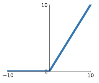
$$ f(x) = \max(0,x) $$
- Pro
- Does not saturate (in +region)
- Very computationally efficient
- Converges much faster than sigmoid/tanh in practive (e.g. 6x)
- Actually more biologically plausible than sigmoid
- Con
- Not Zero-centered output
- An annoyance: (for x<0, dead ReLU will never activate => never update)
Leaky ReLU [Mass et al., 2013] [He et al., 2015]
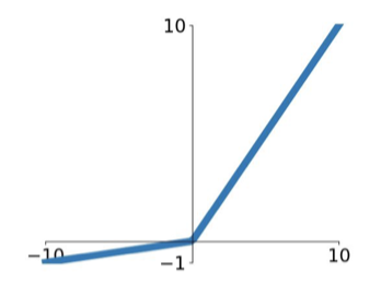
$$ f(x) = \max(0.01x,x) $$
- Pro
- Does not saturate
- Computationally efficient
- Converges much faster than sigmoid/tanh in proctice! (e.g. 6x)
- will not “die”.
- Con
- Not Zero-centered output
- Parametric Rectifier (PReLU)
$$ f(x) = \max(\alpha x, x) $$ where $\alpha$ is a parameter that we can backprop into and lean.
Exponential Linear Units (ELU) [Clevert et al., 2015]
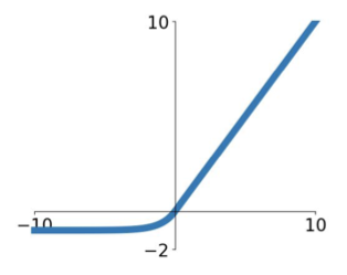
$$ f(x) = \begin{cases} \begin{align} &x & \text{if } x\geq0 \\ &\alpha =(\exp(x)-1) & \text{if } x\leq0 \end{align} \end{cases} $$
- Pro
- All benefits of ReLU
- Closer to zero mean outpus
- Negative saturation regime compared with Leaky ReLU adds some robustness to noise
- Con
- Computation requires exp()
Maxout “Neuron” [Goodfellow et al., 2013]
$$ f(x) = \max(\omega_1^Tx+b_1,\omega_2^T+b_2) $$
- Pro
- Does not have the basic form of dot product -> nonlinearity
- Generalizes ReLU and Leaky ReLU
- Linear Regime! Does not saturate! Does not die!
- Con
- doubles the number of parameters/neuron :(
TLDR: In practiec:
- Use ReLU. Be careful with your learning rates
- Try out Leaky ReLU / Maxout / ELU
- Try out tanh but don’t expect much
- Don’t use sigmoid
1.2 Data Preprocessing
TLDR: In practice for images: center only
- Subtract the mean image (e.g. AlexNet) It is used in original ResNet paper, see reference here.
- Subtract per-channel mean (e.g. VGGNet)
- Not common to normalize variance, to do PCA or whitening
这里减去图像的平均值操作,于我而言,非常诡异。相当于是对结构化数据的每个特征进行去均值操作,对于图像来说就是每张图片相对应的像素点位置的值。
这种操作其实非常局域化,该操作成功的前提是训练集里的图片分布完全符合真实未知的图像分布,所以训练集上算出来的“均值”图像才能当做非常一般化的工具对测试集等未知图片进行去均值。
下图是在下一讲中,小哥多给了一个例子的讲解:
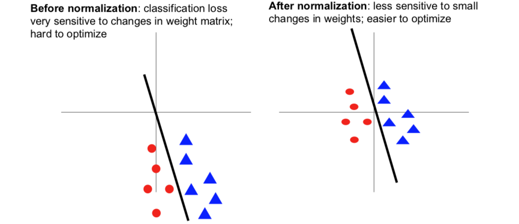
这告诉我们:
(左图)中损失函数对我们的权重矩阵中的线性分类器中的小扰动非常敏感。虽然也可以得到相同的函数,但这会让深度学习变得异常艰难,因为损失对我们的参数向量非常敏感。(右图)将数据点移动到原点附近,并且缩小它们的单位方差,我们仍然可以很好的对这些数据进行分类,但现在当我们稍微的转动直线,我们的损失函数对参数值中的小扰动就不那么敏感了。这可能会优化变得更容易一些的同时能够进展。
顺便提及的是,这种情况不仅仅在线性分类中遇到,记住!在神经网络中,我们需要交叉地使用线性矩阵相乘或者卷积还有非线性激活函数。如果神经网络中某一层的输入均值不为0,或者方差不为1,该层网络权值矩阵的微小摄动就会造成该层输出的巨大摄动,从而造成学习困难。所以这就直观地解释了为什么归一化那么重要。
还要记住,因为我们了解了归一化的重要性,所以引入了 batch normalization 的概念。以使得中间的激活层均值为0,方差为1。(后面会详细介绍)
1.3 Weight Initialization
首先为了打破参数对称问题,参数初始化不能为全部为0(也不能为常数)。
Small random number (gaussian with zero mean and 1e-2 standard deviation)
W = 0.01 * np.random.randn(D, H)Work ~okey for small networks, but problems with deeper networks.
对于层数很多的神经网络,all activations become zero!对于反向传播时,相应的权重梯度也会非常非常小。
我现在知道为啥我的 CNN 层数越多到一定程度(5层以上),网络的性能就开始饱和,甚至开始下降了,这很可能和参数初始化有一定的关系。
如果将高斯分布的方差增大一些(如 1.0)
W = np.random.randn(fan_in, fan_out) * 1.0 # layer initialization会发现:Almost all neurons completely saturated, eigher -1 and 1. Gradients will be all zero.
Reasonable initialization (Mathematical derivation assumes linear activations)
W = np.random.randn(fan_in, fan_out) / np.sqrt(fan_in) # layer initialization“Xavier initialization” [Glorot et al., 2010]
这种初始化方式对于 Tanh 非线性激活,效果不错,每一层都差不多是一个不错的高斯分布。但是!
But when using ReLU nonlinearity it breaks. 一半的神经元会被砍掉。
W = np.random.randn(fan_in, fan_out) / np.sqrt(fan_in/2) # layer initialization[He et al., 2015] (note additional
/2) 这种初始化可以很好的解决,深度神经网络的每层会有一个单位高斯分布。
Slice 中用来可视化不同参数初始化的代码似乎非常棒!贴在这里,以备不时之需!
# assume some unit gaussian 10-D input data
D = np.random.randn(1000, 500)
hidden_layer_sizes = [500] * 10
nonlinearities = ['tanh'] * len(hidden_layer_sizes)

act = {'relu': lambda x:np.maximum(0,x), 'tanh': lambda x:np.tanh(x)}
Hs = {}
for i in range(len(hidden_layer_sizes)):
    X = D if i == 0 else Hs[i-1] # input at this layer
    fan_in = X.shape[1]
    fan_out = hidden_layer_sizes[i]
    W = np.random.randn(fan_in, fan_out) * 0.01 # layer initialization

    H = np.dot(H, W) # matrix multiply
    H = act[nonlinearities[i]](H) # nonlinearity
    Hs[i] = H # cache result on this layer

# look at distributions at each layer
print('input layer had mean %f and std %f' % (np.mean(D), np.std(D)))
layer_means = [np.mean(H) for i, H in Hs.iteritems()]
later_stds = [np.std(H) for i, H in Hs.interitems()]
for i, H in Hs.iteritems():
    print('hidden layer %d had mean %f and std %f' %(i+1, layer_means[i], layer_stds[i]))

# plot the means and standard deviations
plt.figure()
plt.subplot(121)
plt.plot(Hs.keys(), layer_means, 'ob-')
plt.title('layer mean')
plt.subplot(122)
plt.plot(Hs.keys(), layer_stds, 'or-')
plt.title('layer std')

# plot the raw distributions
plt.figure()
for i, H in Hs.iteritems():
    plt.subplot(1, len(Hs), i+1)
    plt.hist(H.ravel(), 30, range=(-1,1))
Proper initialization is an active area of reasearch…
- Understanding the difficulty of training deep feedforward neural networks by Glorot and Bengio, 2010 [PDF]
- Exact solutions to the nonlinear dynamics of learning in deep linear neural networks by Saxe et al, 2013 [PDF]
- Random walk initialization for training very deep feedforward networks by Sussillo and Abbott, 2014 [PDF]
- Delving deep into rectifiers: Surpassing human-level performance on ImageNet classification by He et al., 2015 [PDF]
- Data-dependent Initializations of Convolutional Neural Networks by Krähenbühl et al., 2015 [PDF]
- All you need is a good init, Mishkin and Matas, 2015 [PDF]
- …
1.4 Batch Normalization
动机:让激活函数都在我们想要的高斯范围内保持激活。
- Original paper:[loffe and Szegedy, 2015]
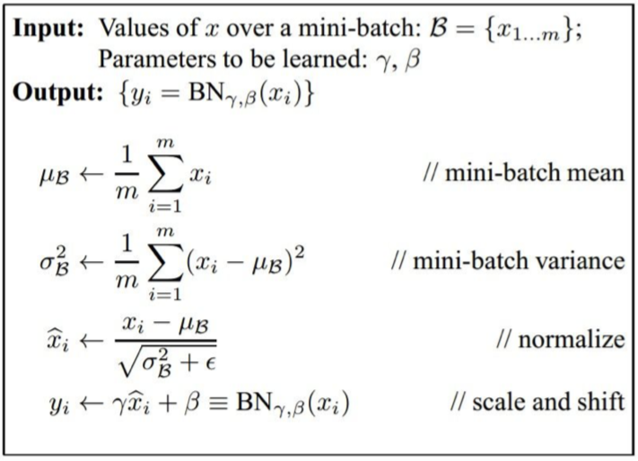
假设我们在当前的 batch 中有 N 个训练样本,并且假设每 batch 是 D 维的。然后,我们将对每个维度纵向独立的计算经验均值(empirical mean)和方差(variance)。所以,基本上每个特征元素(每特征图对应位置的值),通过这种小批量处理都进行计算,并且对其进行归一化:
$$ \hat{x}^{(k)}=\frac{x^{(k)}-E[x^{(k)}]}{\sqrt{\text{Var}[x^{(k)}]}},. $$
要把 BN 层放在哪里呢?
- 通常放在全连接层之后,或者卷积计算层之后,非线性激活层之前。
其实我们可以不用那么太严格的高斯分布,只要让神经元听话点就行了。所以,我们给 BN 层加一个可调节效果程度的“开关”,作为网络模型可学习参数的一部分,使得让网络自己学习控制让激活函数具有更高或更低的饱和度的能力,具有灵活性。废话说那么多,就是再加一个式子,允许网络自行压缩/平移输出值的范围: $$ y^{(k)}=\gamma^{(k)}\hat{x}^{(k)}+\beta^{(k)} $$ 其中,待学习的参数分别为 $\gamma^{(k)}=\sqrt{\text{Var}[x^{(k)}]},\beta^{(k)}=\text{E}[x^{(k)}]$ 时,可以回到未加 BN 层的恒等映射。(但在实践中,这种极端情况并不会真的出现;而且,加上 BN 层后,输出值只能说大约相近于高斯分布,实践中并不必完全符合;还有需要提及的是,在测试的时候,我们并不需要每次去计算这个均值和方差了,只需要训练集中记录好的平均偏移量(running averages)来计算即可)
总结一下:
好处:
- Improves gradient flow through the network (这是动机)
- Allows higher learning rates
- Reduces the strong dependence on initialization (这是动机)
- 更高的鲁棒性
- Acts as a form of regularization in a funny way, and slightly reduces the need for dropout, maybe
2. Training dynamics
下面,我们要讨论的是:如何监视训练过程。
2.1 Babysitting the Learning Process
Preprocess the data
数据预处理,使得每个对应像素点值标准化:
X -= np.mean(X, axis = 0)
X /= np.std(X, axis = 0)
Choose the architecture
- 这没啥可说的,确定好你的网络就是了。
Double check that the loss is reasonable
完整性检查:(first iteration)
- 无正则化时,损失值符合预期
- 有正则化时,损失值有略微的提升
- 取非常少量的训练样本作为训练集训练,无正则化,用最简单的 SGD 优化。目标是:过拟合!
接下来就可以开始正式训练了~!
用全部的训练集样本训练,很小的正则化,使用一个较小的学习率开始训练。
如果损失值几乎没有变动,说明学习率太低了。不过要是你看到训练/测试上的 accuracy 在提升,说明参数梯度更新方向是对的。
如果损失值是 NaN,就是学习率很可能是太低了。粗略地说,学习率应该是在 (1e-3…1e-5) 的交叉验证范围内。
2.2 Hyperparameter Optimization
刚刚稍微涉及了一点学习率的调参问题,现在开始全面的谈一谈。
多的先不说,要交叉验证!(额。。。真的要交叉验证么?)
首先,非常分散的取几个超参数的值,然后用几个 epoch 的迭代去学习,确保那些超参数是起码能用的。并且挑出验证集上准确率较高的一套超参数的范围。
(Tip:如果某次迭代的损失值已经超过第一次迭代的3倍了,那就果断放弃这套参数吧!)
第二步,进一步划小超参数的范围训练吧!longer running time, finer search … (repeat as necessary)
(Tip:正则和学习率两个超参数的交叉验证取值可以采用10的对数之间均匀采样为好,因为学习率在梯度更新时具有乘法效应。可如下设置超参数:
reg = 10**uniform(-5, 5)
lr = 10*uniform(-3, -6)
)
(Tip:在进一步划定小的超参数区间去进一步交叉验证时,要避免出现较好的验证结果都出现在超参数的采样边缘。)
(Tip:可以考虑用随机搜索代替网格搜索。[Random Search for Hyper-Parameter Optimization - Bergstra and Bengio, 2012]。这是因为对于超过一个变量的函数而言,随机采样会更加真实。通常我们会对我们真正有的维度进行稍微的有效的降维,接着就可以得到更多已有的重要变量的样本,进而就能得到更多有用的信息)
(小哥对随机搜索在理论上的优越性解释:因为当你的模型性能对某一个超参数比对其他超参数更敏感的时候,随机搜索可以对超参数空间覆盖的更好。)
(小哥对粗细粒交叉搜索的解释:当你做超参数优化的时候,一开始可能会处理很大的搜索范围,几次迭代之后就可以缩小范围,圈定合适的超参数所在的区域,然后再对这个小范围重复这个过程。你可以多次迭代进行上述的步骤,已获得超参数的正确区域。另外很重要的一点是,一开始你得确定粗略的范围,这个范围要非常宽,覆盖你所有的超参数。理想情况下,范围应该足够宽到你的网络不会超过范围的任何另一边。这样你就知道自己的搜索范围足够大。)
(小哥的FYI解答:通常最先定下的超级敏感的学习率!然后才是正则化啦,网络结构啦等等)
超参数调参之路是永无止境的!还有很多要调,比如:
- network architecture
- learning rate, its decay schedule, update type
- regularization (L2/Dropout strength)
- ….
你!就是未来玩转深度学习的著名 DJ 手!

More Tips:
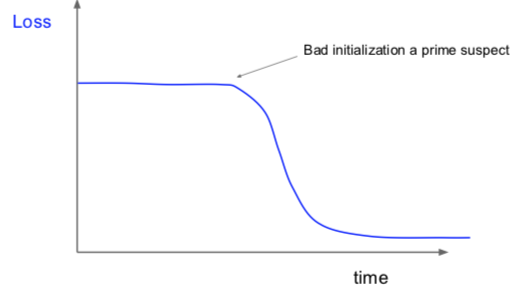
如果损失值刚开始的时候很平滑,然后突然开始训练的话,很可能说明权重参数初始值不够好。
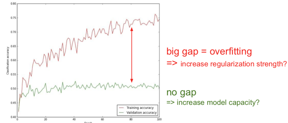
留意训练迭代过程中的 accuracy:
应该记录权重的更新值和更新的幅度变化:
# assume parameter vector W and its gradient vector dW
param_scale = np.linalg.norm(W.ravel())
update = - learning_rate * dW # simple SGD update
update_scale = np.linalg.norm(update.revel())
W += update # the actual update
print(update_scale / param_scale) # want ~1e-3
ratio between the updates and values: ~ 0.0002 / 0.02 = 0.01 (about okay)
want this to be somewhere around 0.001 or so