 Image credit: LIGO-G2001862. Reproduced by Herb.
数据来源 (Data Sources):
LIGO-Virgo Cumulative Event Rate Plot O1-O3a (added a separate plot to include O3b public alerts)
- LIGO-G2001862-v3 (Public)
- LIGO-G2001862-v3 (Private)
Note that G1901322 contains confirmed events and public alerts. And original cumulative event rate plot was coded in MATLAB.
Loading packages and data
import numpy as np
import datetime
import matplotlib.pyplot as plt

gw_event = [20150914,20151012,20151226, # O1 events
    20170104,20170608,20170729,20170809,20170814,20170817,20170818,20170823,
    20190408,20190412,20190413,20190413,20190421,20190424,20190425,20190426,
    20190503,20190512,20190513,20190514,20190517,20190519,20190521,20190521,
    20190527,20190602,20190620,20190630,20190701,20190706,20190707,20190708,
    20190719,20190720,20190727,20190728,20190731,20190803,20190814,20190828,
    20190828,20190909,20190910,20190915,20190924,20190929,20190930, # gap between O3a and O3b
    20191105,20191109,20191129,20191204,20191205,20191213,20191215,
    20191216,20191222,20200105,20200112,20200114,20200115,20200128,20200129,
    20200208,20200213,20200219,20200224,20200225,20200302,20200311,20200316];
assert sorted(gw_event) == gw_event

datetime_event = [datetime.datetime.strptime(str(t), '%Y%m%d') for t in gw_event]
# Know more about Format Codes? see: https://docs.python.org/zh-cn/3/library/datetime.html#strftime-strptime-behavior

num_event = len(datetime_event)
print('Total number of GW events:', num_event)
Total number of GW events: 73
Pre-processing the data for drawing
O1_start = datetime.datetime(2015,9,12)
O1_end = datetime.datetime(2016,1,19)
len_O1 = O1_end - O1_start

O2_start = datetime.datetime(2016,11,30)
O2_end = datetime.datetime(2017,8,25)
len_O2 = O2_end - O2_start

O3a_start = datetime.datetime(2019,4,1)
O3a_end   = datetime.datetime(2019,9,30)
len_O3a = O3a_end - O3a_start

O3b_start = datetime.datetime(2019,11,1)
O3b_end   = datetime.datetime(2020,4,30)
len_O3b = O3b_end - O3b_start

total_days = len_O1 + len_O2 + len_O3a + len_O3b
O1  = len_O1
O2  = len_O1 + len_O2
O3a = len_O1 + len_O2 + len_O3a
O3b = len_O1 + len_O2 + len_O3a + len_O3b

nev_O1 = sum((O1_start <= np.asarray(datetime_event)) & (np.asarray(datetime_event) <= O1_end))
nev_O2 = sum((O2_start <= np.asarray(datetime_event)) & (np.asarray(datetime_event) <= O2_end))
nev_O3a = sum((O3a_start <= np.asarray(datetime_event)) & (np.asarray(datetime_event) <= O3a_end))
nev_O3b = sum((O3b_start <= np.asarray(datetime_event)) & (np.asarray(datetime_event) <= O3b_end))
assert num_event == nev_O1 + nev_O2 + nev_O3a + nev_O3b

print('Total of days:', total_days.days)
print('Number of days in O1/O2/O3a/O3b:', '{}/{}/{}/{}'.format(len_O1.days,len_O2.days,len_O3a.days,len_O3b.days))
print('Number of events in O1/O2/O3a/O3b:', '{}/{}/{}/{}'.format(nev_O1, nev_O2, nev_O3a, nev_O3b))
Total of days: 760
Number of days in O1/O2/O3a/O3b: 129/268/182/181
Number of events in O1/O2/O3a/O3b: 3/8/39/23
Figure: Cumulative Count of GW Events by dates.
plt.figure(figsize=(8,4))
plt.hist(datetime_event,  bins=73,  histtype='step', cumulative=True, color='k', linewidth=2)
plt.ylabel('Cumulative #Events/Candidates')
plt.fill_betweenx([-1,80], O1_start,O1_end , color=[230/256,179/255,179/255])
plt.fill_betweenx([-1,80], O2_start,O2_end , color=[179/256,230/255,181/255])
plt.fill_betweenx([-1,80], O3a_start,O3a_end , color=[179/256,179/255,228/255])
plt.fill_betweenx([-1,80], O3b_start,O3b_end , color=[255/256,179/255,84/255])
plt.ylim(-1,80)
plt.xlim(O1_start, O3b_end)
plt.title('''Cumulative Count of Events and (non-retracted Alerts)
O1={}, O2={}, O3a={}, O3b={}, Total={}'''.format(nev_O1,nev_O2,nev_O3a,nev_O3b,num_event))
plt.savefig('cumulative_events_by_date.png', dpi=300, bbox_inches='tight')
plt.show()
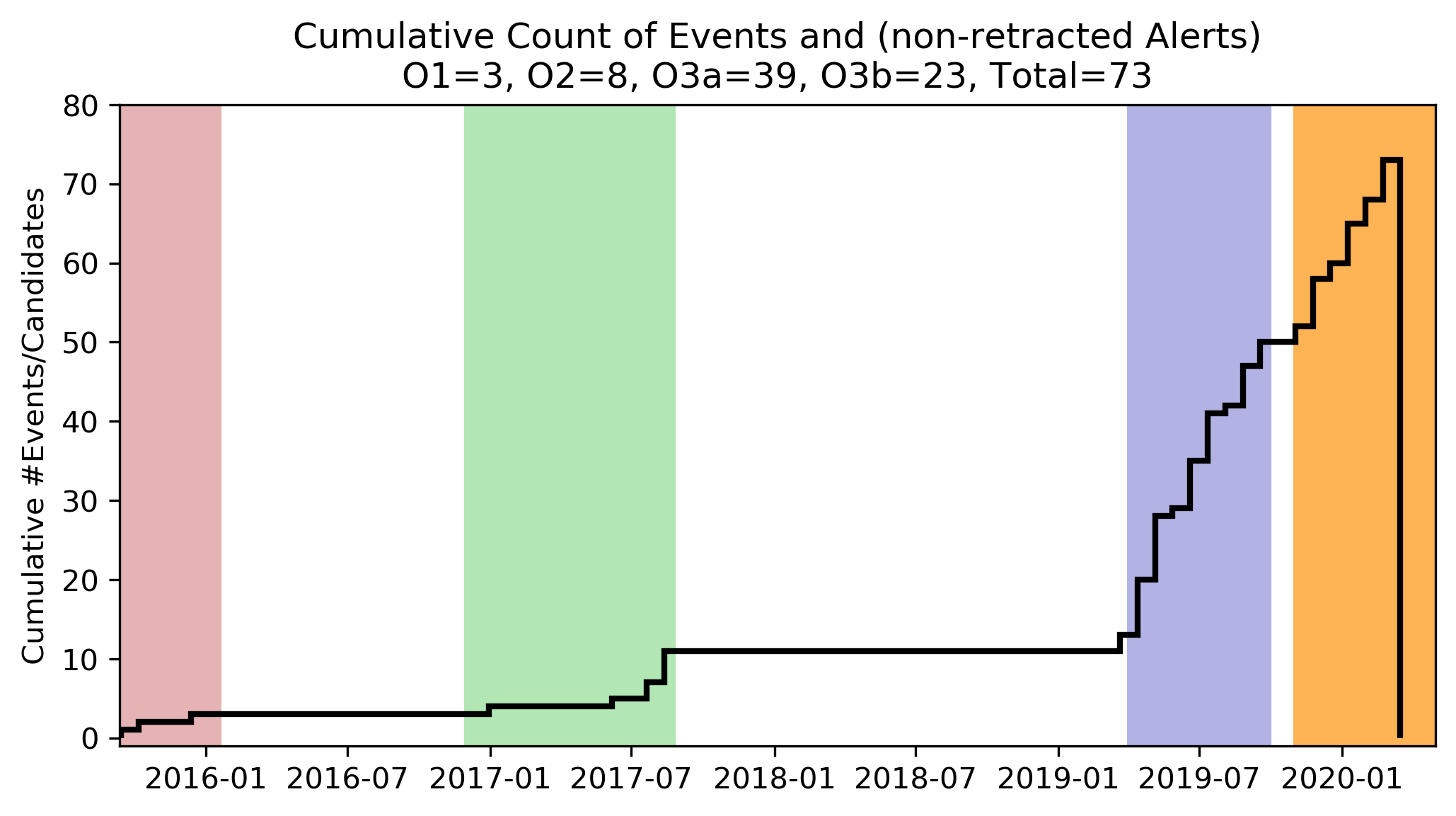
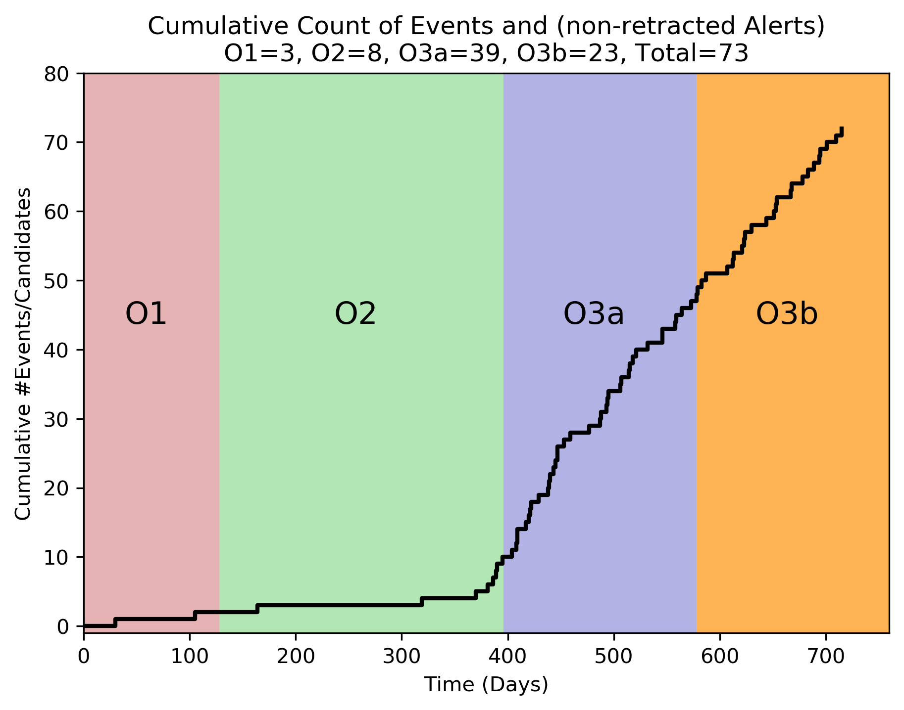
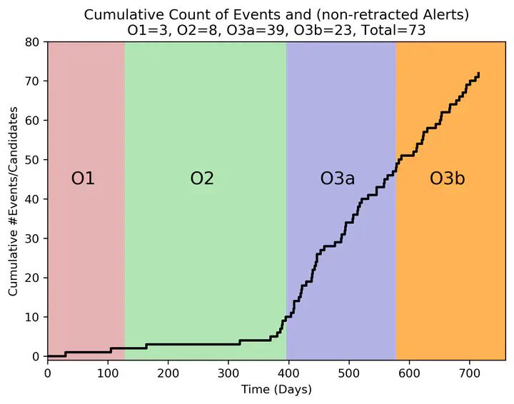
Figure: Cumulative Count of GW Events by days of running for each event.
def getstart(t):
    if (O1_start <= t) & (t <= O1_end):
        return O1_start
    elif (O2_start <= t) & (t <= O2_end):
        return O2_start - O1
    elif (O3a_start <= t) & (t <= O3a_end):
        return O3a_start - O2
    elif (O3b_start <= t) & (t <= O3b_end):
        return O3b_start - O3a
    else:
        raise
x = [ (t-getstart(t)).days for t in datetime_event]
y = range(len(datetime_event))

plt.figure(figsize=(7,5))
plt.plot(x, y, drawstyle='steps-post', color='k', linewidth=2)
plt.fill_betweenx([-1,80], 0, O1.days , color=[230/256,179/255,179/255])
plt.fill_betweenx([-1,80], O1.days, O2.days , color=[179/256,230/255,181/255])
plt.fill_betweenx([-1,80], O2.days, O3a.days , color=[179/256,179/255,228/255])
plt.fill_betweenx([-1,80], O3a.days, O3b.days , color=[255/256,179/255,84/255], )
plt.ylim(-1,80)
plt.xlim(0, O3b.days)
plt.ylabel('Cumulative #Events/Candidates')
plt.xlabel('Time (Days)')
plt.title('''Cumulative Count of Events and (non-retracted Alerts)
O1={}, O2={}, O3a={}, O3b={}, Total={}'''.format(nev_O1,nev_O2,nev_O3a,nev_O3b,num_event))
plt.text(O1.days*0.3, num_event*0.6, 'O1', fontsize=15)
plt.text(O1.days+(O2.days-O1.days)*0.4, num_event*0.6, 'O2', fontsize=15)
plt.text(O2.days+(O3a.days-O2.days)*0.3, num_event*0.6, 'O3a', fontsize=15)
plt.text(O3a.days+(O3b.days-O3a.days)*0.3, num_event*0.6, 'O3b', fontsize=15)
plt.savefig('cumulative_events_by_days.png', dpi=300, bbox_inches='tight')
plt.show()