Bayes Inference, Bayes Factor, Model Selection

---

Bayes Inference

A primary aim of modern Bayesian inference is to construct a posterior distribution $$ p(\theta|d) $$ where $\theta$ is the set of model parameters and $d$ is the data associated with a measurement¹. The posterior distribution $p(\theta|d)$ is the probability density function for the continuous variable $\theta$ (i.e. 15 parameters describing a CBC) given the data $d$ (strain data from a network of GW detectors). The probability that the true value of $\theta$ is between $(\theta’,\theta’+d\theta)$ is given by $p(\theta’|d)d\theta’$. It is normalised so that $$ \int d\theta p(\theta|d) = 1 . $$

According to Bayes theorem, the posterior distribution for multimessenger astrophysics is given by $$ p(\theta \mid d)=\frac{\mathcal{L}(d \mid \theta) \pi(\theta)}{\mathcal{Z}} $$ where $\mathcal{L}(d \mid \theta)$ is the likelihood function of the data given the $\theta$, $\pi(\theta)$ is the prior distribution of $\theta$, and $\mathcal{Z}$ is a normalisation factor called the ‘evidence’: $$ \mathcal{Z} \equiv \int d \theta \mathcal{L}(d \mid \theta) \pi(\theta) . $$

The likelihood function is something that we choose. It is a description of the measurement. By writing down a likelihood, we implicitly introduce a noise model. For GW astronomy, we typically assume a Gaussian-noise likelihood function that looks something like this $$ \mathcal{L}(d \mid \theta)=\frac{1}{\sqrt{2 \pi \sigma^{2}}} \exp \left(-\frac{1}{2} \frac{(d-\mu(\theta))^{2}}{\sigma^{2}}\right) , $$ where $\mu(\theta)$ is a template for the gravitational strain waveform given $\theta$ and $\sigma$ is the detector noise. Note the $\pi$ with no parantheses and no subscript is the mathematical constent, not a prior distribution. This likelihood function reflects our assumption that the noise in GW detctors is Gaussian. Note that the likelihood function is not normalised with respect the $\theta$ and so $\int d\theta\mathcal{L}(d|\theta)\neq1$.

In practical terms, the evidence is a single number. It usually does not mean anything by itself, but becomes useful when we compare one evidence with another evidence. Formally, the evidence is a likelihood function. Specifically, it is the completely marginalised likelihood function. It is therefore sometimes denoted $\mathcal{L}(d)$ with no $\theta$ dependence. However, we prefer to use $\mathcal{Z}$ to denote the fully marginalised likelihood function.

---

Bayes Factor

The ratio of the evidence for two different models is called the Bayes factor. For example, we can compare the evidence for a BBH waveform predicted by general relativity (model $M_A$ with parameters $\theta$ ) with a BBH waveform predicted by some other theory (model $M_B$ with parameters $\nu$): $$ \begin{aligned} \mathcal{Z}_{A}&=\int d \theta \mathcal{L}\left(d \mid \theta, M_{A}\right) \pi(\theta) ,\\ \mathcal{Z}_{B}&=\int d \nu \mathcal{L}\left(d \mid \nu, M_{B}\right) \pi(\nu) . \end{aligned} $$ The A/B Bayes factor is $$ \mathrm{BF}_{B}^{A}=\frac{\mathcal{Z}_{A}}{\mathcal{Z}_{B}} . $$ Note that the number of parameters in $\nu$ can be different from the number of parameters in $\theta$.

Formally, the correct metric to compare two models is not the Bayes factor, but rather the odds ratio. The odds ratio is the product of the Bayes factor with the prior odds $\pi_A/\pi_B$, which describes our likelihood of hypotheses $A$ and $B$: $$ \mathcal{O}_{B}^{A} \equiv \frac{\mathcal{Z}_{A}}{\mathcal{Z}_{B}} \frac{\pi_{A}}{\pi_{B}} =\frac{\pi_{A}}{\pi_{B}} \mathrm{BF}_{B}^{A} $$

In many practical applications, we set the prior odds ratio to unity, and so the odds ratio is the Bayes factor. This practice is sensible in many applications where our intuition tells us: until we do this measurement both hypotheses are equally likely.

There are some (fairly uncommon) examples where we might choose a different prior odds ratio. For example, we may construct a model in which general relativity (GR) is wrong. We may further suppose that there are multiple different ways in which it could be wrong, each corresponding to a different GR-is-wrong sub-hypothesis. If we calculated the odds ratio comparing one of these GR-is-wrong sub-hypotheses to the GR-is-right hypothesis, we would not assign equal prior odds to both hypotheses. Rather, we would assign at most 50% probability to the entire GR-is-wrong hypothesis, which would then have to be split among the various sub-hypotheses.

---

Model Selection

Bayesian evidence encodes two pieces of information:

1. The likelihood tells us how well our model fits the data.
2. The act of marginalisation tell us about the size of the volume of parameter space we used to carry out a fit.

This creates a sort of tension:

We want to get the best fit possible (high likelihood) but with a minimum prior volume.

A model with a decent fit and a small prior volume often yields a greater evidence than a model with an excellent fit and a huge prior volume.

In these cases, the Bayes factor penalises the more complicated model for being too complicated.

We can obtain some insights into the model evidence by making a simple approximation to the integral over parameters:

• Consider first the case of a model having a single parameter $w$. ($N=1$)
• Assume that the posterior distribution is sharply peaked around the most probable value $w_\text{MAP}$, with width $\Delta w_\text{posterior}$, then we can approximate the in- tegral by the value of the integrand at its maximum times the width of the peak.
• Assume that the prior is flat with width $\Delta w_\text{prior}$ so that $\pi(w) = 1/\Delta w_\text{prior}$.

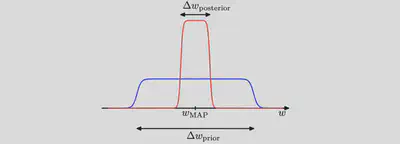
then we have $$ \mathcal{Z} \equiv \int d w \mathcal{L}(d \mid w) \pi(w) \simeq \mathcal{L}\left(\mathcal{d} \mid w_{\mathrm{MAP}}\right) \frac{\Delta w_{\text {posterior }}}{\Delta w_{\text {prior }}} $$ and so taking logs we obtain (for a model having a set of $N$ parameters) $$ \ln \mathcal{Z}(\mathcal{d}) \simeq \ln \mathcal{L}\left(\mathcal{d} \mid w_{\mathrm{MAP}}\right)+N\ln \left(\frac{\Delta w_{\text {posterior }}}{\Delta w_{\text {prior }}}\right) $$

• The first term: the fit to the data given by the most probable parameter values, and for a flat prior this would correspond to the log likelihood.
• The second term (also called Occam factor) penalizes the model according to its complexity. Because $\Delta w_\text{posterior}<\Delta w_\text{prior}$ this term is negative, and it increases in magnitude as the ratio $\Delta w_\text{posterior}/\Delta w_\text{prior}$ gets smaller. Thus, if parameters are finely tuned to the data in the posterior distribution, then the penalty term is large.

Thus, in this very simple approximation, the size of the complexity penalty increases linearly with the number $N$ of adaptive parameters in the model. As we increase the complexity of the model, the first term will typically decrease, because a more complex model is better able to fit the data, whereas the second term will increase due to the dependence on $N$. The optimal model complexity, as determined by the maximum evidence, will be given by a trade-off between these two competing terms. We shall later develop a more refined version of this approximation, based on a Gaussian approximation to the posterior distribution.

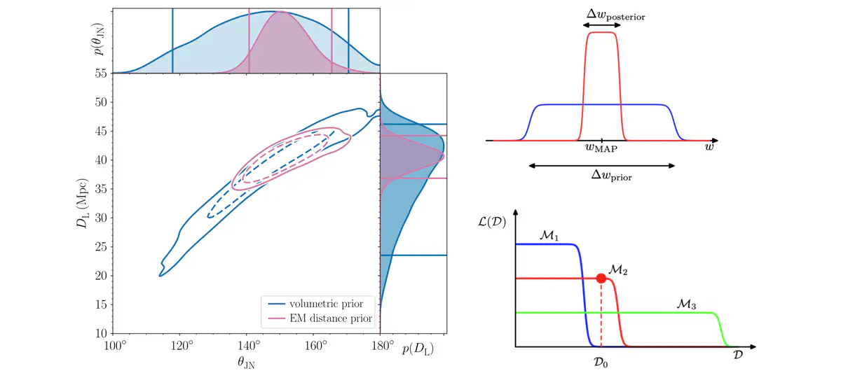
A further insight into Bayesian model comparison and understand how the marginal likelihood can favour models of intermediate complexity by considering the Figure below.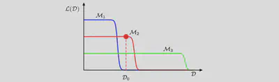

Here the horizontal axis is a one-dimensional representation of the space of possible data sets, so that each point on this axis corresponds to a specific data set. We now consider three models $M_1$, $M_2$ and $M_3$ of successively increasing complexity. Imagine running these models generatively to produce example data sets, and then looking at the distribution of data sets that result. Any given model can generate a variety of different data sets since the parameters are governed by a prior probability distribution, and for any choice of the parameters there may be random noise on the target variables. To generate a particular data set from a specific model, we first choose the values of the parameters from their prior distribution $\pi(w)$, and then for these parameter values we sample the data from $\mathcal{L}(\mathcal{D}|w)$. Because the distributions $\mathcal{L}(\mathcal{D}|M_i)$ are normalized, we see that the particular data set $D_0$ can have the highest value of the evidence for the model of intermediate complexity. Essentially, the simpler model cannot fit the data well, whereas the more complex model spreads its predictive probability over too broad a range of data sets and so assigns relatively small probability to any one of them.

More insights:

• If we compare two models where one model is a superset of the other—for example, we might compare GR and GR with non-tensor modes—and if the data are better explained by the simpler model, the log Bayes factor is typically modest, $$ |\log \mathrm{BF}| \approx (1,2). $$ Thus, it is difficult to completely rule out extensions to existing theories. We just obtain ever tighter constraints on the extended parameter space.

• To make good use of Bayesian model comparison, we fully specify priors that are independent of the current data $\mathcal{D}$.

• The sensitivity of the marginal likelihood to the prior range depends on the shape of the prior and is much greater for a uniform prior than a scale-invariant prior (see e.g. Gregory, 2005b, 61).

• In most instances we are not particularly interested in the Occam factor itself, but only in the relative probabilities of the competing models as expressed by the Bayes factors. Because the Occam factor arises automatically in the marginalisation procedure, its effects will be present in any model-comparison calculation.

• No Occam factors arise in parameter-estimation problems. Parameter estimation can be viewed as model comparison where the competing models have the same complexity so the Occam penalties are identical and cancel out.

• On average the Bayes factor will always favour the correct model.

  To see this, consider two models $\mathcal{M}_\text{true}$ and $\mathcal{M}_1$ in which the truth corresponds to $\mathcal{M}_\text{true}$. We assume that the true posterior distribution from which the data are considered is contained within the set of models under consideration. For a given finite data, it is possible for the Bayes factor to be larger for the incorrect model. However, if we average the Bayes factor over the distribution of data sets, we obtain the expected Bayes factor in the form $$ \int \mathcal{Z}\left(\mathcal{D} \mid \mathcal{M}_{true}\right) \ln \frac{\mathcal{Z}\left(\mathcal{D} \mid \mathcal{M}_{true}\right)}{\mathcal{Z}\left(\mathcal{D} \mid \mathcal{M}_{1}\right)} \mathrm{d} \mathcal{D} $$ where the average has been taken with respect to the true distribution of the data. This is an example of Kullback-Leibler divergence and satisfies the property of always being positive unless the two distributions are equal in which case it is zero. Thus on average the Bayes factor will always favour the correct model.

We have seen from Figure 1 that the model evidence can be sensitive to many aspects of the prior, such as the behaviour in the tails. Indeed, the evidence is not defined if the prior is improper, as can be seen by noting that an improper prior has an arbitrary scaling factor (in other words, the normalization coefficient is not defined because the distribution cannot be normalized). If we consider a proper prior and then take a suitable limit in order to obtain an improper prior (for example, a Gaussian prior in which we take the limit of infinite variance) then the evidence will go to zero, as can be seen Figure 1 and the equation below the Figure 1. It may, however, be possible to consider the evidence ratio between two models first and then take a limit to obtain a meaningful answer.

In a practical application, therefore, it will be wise to keep aside an independent test set of data on which to evaluate the overall performance of the final system.

---

Reference

• An introduction to Bayesian inference in gravitational-wave astronomy: Parameter estimation, model selection, and hierarchical models

  Eric Thrane, Colm Talbot

  Cite DOI
• Pattern recognition and machine learning

  Christopher M Bishop

  Cite
• Bayesian astrophysics

  Andrés Asensio Ramos, Iñigo Arregui

  Cite