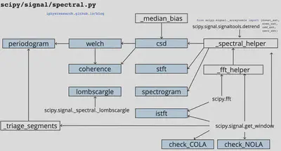
SciPy (pronounced “Sigh Pie”) is open-source software for mathematics, science, and engineering. It includes modules for statistics, optimization, integration, linear algebra, Fourier transforms, signal and image processing, ODE solvers, and more.
# Preparingmode='stft'# or psdsame_data=Trueoutdtype=np.result_type(x,np.complex64)# 明确数据精度axis=-1window='hann'boundary='zeros'padded=True# not useddetrend=False# not usedscaling='spectrum'# or densityreturn_onesided,sides=True,'onesided'fromscipy.signal._arraytoolsimportconst_ext,even_ext,odd_ext,zero_extboundary_funcs={'even':even_ext,'odd':odd_ext,'constant':const_ext,'zeros':zero_ext,None:None}
boundary_funcs 是考虑对数据 x 将会以什么样的形式来延拓其边界。后面很快会再讨论到这一点。
Finetune
下面的参数是比较重要的可调参数:
## Finetune ## # parse window; nperseg = win.shapenperseg=nperseg=fs//4nperseg=int(nperseg)print('nperseg = {}'.format(nperseg))# parse window; if array like, then set nperseg = win.shapewin,nperseg=signal.spectral._triage_segments(window,nperseg,input_length=x.shape[-1])print('nperseg = {}, win.size = {}'.format(nperseg,win.size))# win have the same dtype with outdtypeifnp.result_type(win,np.complex64)!=outdtype:win=win.astype(outdtype)# nfft must be greater than or equal to nperseg.nfft=int(fs//4)print('nfft = {}'.format(nfft))# noverlap must be less than nperseg.noverlap=int(fs//8)print('noverlap = {}'.format(noverlap))nstep=nperseg-noverlapprint('nstep = {}'.format(nstep))## output ### nperseg = 4096# nperseg = 4096, win.size = 4096# nfft = 4096# noverlap = 2048# nstep = 2048
nperseg 表示的是要解析的短时窗口序列的长度 (number of per segment)。
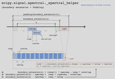
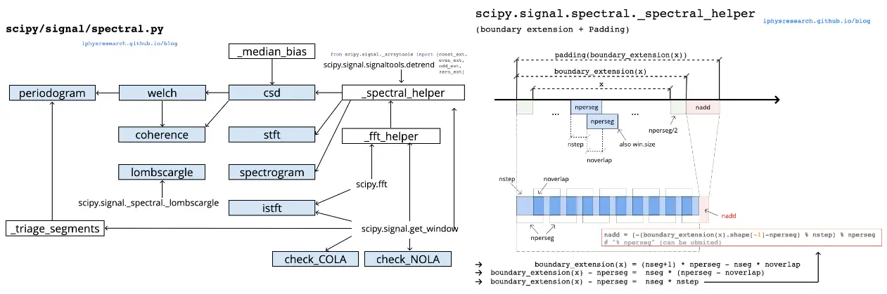
正式计算之前,还需要对我们的完整数据 x 进行边界延拓和补零的操作。下面的注释中也给出了这样操作偶的理由。
# Padding occurs after boundary extension, so that the extended signal ends# in zeros, instead of introducing an impulse at the end.# I.e. if x = [..., 3, 2]# extend then pad -> [..., 3, 2, 2, 3, 0, 0, 0]# pad then extend -> [..., 3, 2, 0, 0, 0, 2, 3]print('x.size = {}'.format(x.size))# boundary extensionx=boundary_funcs[boundary](x,nperseg//2,axis=-1)print('x.size = {} | {}'.format(x.size,hp.size+nperseg))# Pad to integer number of windowed segments# I.e make x.shape[-1] = nperseg + (nseg-1)*nstep, with integer nsegnadd=(-(x.shape[-1]-nperseg)%nstep)%npersegzeros_shape=list(x.shape[:-1])+[nadd]x=np.concatenate((x,np.zeros(zeros_shape)),axis=-1)print('x.size = {} | {}'.format(x.size,x.size%nperseg))## output ### x.size = 32613# x.size = 36709 | 36709# x.size = 36864 | 0
# Perform the windowed FFTsresult=_fft_helper(x,win,detrend_func,nperseg,noverlap,nfft,sides)def_fft_helper(x,win,detrend_func,nperseg,noverlap,nfft,sides):pass# ... (暂略)returnresult
Scipy 中原代码的实现其实非常 pythonic 风格的方法,那就是将数据 x 映射为一个数据矩阵,每行为每一个待处理的数据 segment,每列都是相同的 nperseg。
Way 1
# Created strided array of data segmentsifnperseg==1andnoverlap==0:result=x[...,np.newaxis]else:# https://stackoverflow.com/a/5568169step=nperseg-noverlapshape=x.shape[:-1]+((x.shape[-1]-noverlap)//step,nperseg)strides=x.strides[:-1]+(step*x.strides[-1],x.strides[-1])result=np.lib.stride_tricks.as_strided(x,shape=shape,strides=strides)
density: Select Power the loss of power is compensated. The ratio of the sum of the squared data before and after applying the window is used as a normalization factor. The total power within the spectrum therefore always corresponds to the power of the data before applying the window.
spectrum: Selecting Amplitude normalizes to the gain of the used window function, i.e. the sum of all values is divided by their number. This compensates the damping of the amplitudes caused by applying the window. This is especially useful to measure peaks within the spectrum.
ifsides=='onesided'andmode=='psd':# not used for stftifnfft%2:result[...,1:]*=2else:# Last point is unpaired Nyquist freq point, don't doubleresult[...,1:-1]*=2# All imaginary parts are zero anywaysifsame_dataandmode!='stft':result=result.real
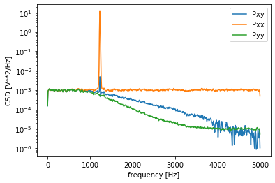
>>>fromscipyimportsignal>>>importmatplotlib.pyplotasplt# Generate two test signals with some common features.>>>fs=10e3>>>N=1e5>>>amp=20>>>freq=1234.0>>>noise_power=0.001*fs/2>>>time=np.arange(N)/fs>>>b,a=signal.butter(2,0.25,'low')>>>x=np.random.normal(scale=np.sqrt(noise_power),size=time.shape)>>>y=signal.lfilter(b,a,x)>>>x+=amp*np.sin(2*np.pi*freq*time)>>>y+=np.random.normal(scale=0.1*np.sqrt(noise_power),size=time.shape)# Compute and plot the magnitude of the cross spectral density.>>>f,Pxy=signal.csd(x,y,fs,nperseg=1024)>>>f,Pxx=signal.csd(x,x,fs,nperseg=1024)>>>f,Pyy=signal.csd(y,y,fs,nperseg=1024)>>>plt.semilogy(f,np.abs(Pxy),label='Pxy')>>>plt.semilogy(f,np.abs(Pxx),label='Pxx')>>>plt.semilogy(f,np.abs(Pyy),label='Pyy')>>>plt.xlabel('frequency [Hz]')>>>plt.ylabel('CSD [V**2/Hz]')>>>plt.legend()>>>plt.show()
其源码的实现:
defcsd(x,y,fs=1.0,window='hann',nperseg=None,noverlap=None,nfft=None,detrend='constant',return_onesided=True,scaling='density',axis=-1,average='mean'):"""Estimate the cross power spectral density, Pxy, using Welch's method."""freqs,_,Pxy=_spectral_helper(x,y,fs,window,nperseg,noverlap,nfft,detrend,return_onesided,scaling,axis,mode='psd')# Average over windows.iflen(Pxy.shape)>=2andPxy.size>0:ifPxy.shape[-1]>1:ifaverage=='median':Pxy=np.median(Pxy,axis=-1)/_median_bias(Pxy.shape[-1])elifaverage=='mean':Pxy=Pxy.mean(axis=-1)else:raiseValueError('average must be "median" or "mean", got %s'%(average,))else:Pxy=np.reshape(Pxy,Pxy.shape[:-1])returnfreqs,Pxy
_median_bias
def_median_bias(n):"""
Returns the bias of the median of a set of periodograms relative to
the mean.
"""ii_2=2*np.arange(1.,(n-1)//2+1)return1+np.sum(1./(ii_2+1)-1./ii_2)
welch (PSD)
Estimate power spectral density using Welch’s method.
Welch’s method 1 computes an estimate of the power spectral density (PSD) by dividing the data into overlapping segments, computing a modified periodogram for each segment and averaging the periodograms.
源码是很简单直接的:
defwelch(x,fs=1.0,window='hann',nperseg=None,noverlap=None,nfft=None,detrend='constant',return_onesided=True,scaling='density',axis=-1,average='mean'):"""Estimate power spectral density using Welch's method."""freqs,Pxx=csd(x,x,fs=fs,window=window,nperseg=nperseg,noverlap=noverlap,nfft=nfft,detrend=detrend,return_onesided=return_onesided,scaling=scaling,axis=axis,average=average)returnfreqs,Pxx.real
这就是所谓的 Welch 方法下的 PSD。看个例子,体会一般:
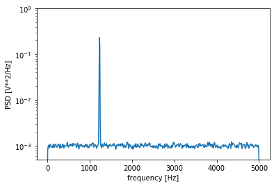
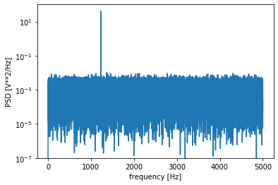
>>>fromscipyimportsignal>>>importmatplotlib.pyplotasplt>>>np.random.seed(1234)# Generate a test signal, a 2 Vrms sine wave at 1234 Hz, corrupted by# 0.001 V**2/Hz of white noise sampled at 10 kHz.>>>fs=10e3>>>N=1e5>>>amp=2*np.sqrt(2)>>>freq=1234.0>>>noise_power=0.001*fs/2>>>time=np.arange(N)/fs>>>x=amp*np.sin(2*np.pi*freq*time)>>>x+=np.random.normal(scale=np.sqrt(noise_power),size=time.shape)
现在来计算并看看这个数据的 PSD,以及噪声的功率密度:
# Compute and plot the power spectral density.>>>f,Pxx_den=signal.welch(x,fs,nperseg=1024)>>>plt.semilogy(f,Pxx_den)>>>plt.ylim([0.5e-3,1])>>>plt.xlabel('frequency [Hz]')>>>plt.ylabel('PSD [V**2/Hz]')>>>plt.show()# If we average the last half of the spectral density, to exclude the# peak, we can recover the noise power on the signal.>>>np.mean(Pxx_den[256:])# 0.0009924865443739191
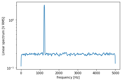
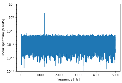
# Now compute and plot the power spectrum.>>>f,Pxx_spec=signal.welch(x,fs,'flattop',1024,scaling='spectrum')>>>plt.figure()>>>plt.semilogy(f,np.sqrt(Pxx_spec))>>>plt.xlabel('frequency [Hz]')>>>plt.ylabel('Linear spectrum [V RMS]')>>>plt.show()# The peak height in the power spectrum is an estimate of the RMS# amplitude.>>>np.sqrt(Pxx_spec.max())# 2.0077340678640727
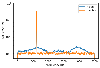
# If we now introduce a discontinuity in the signal, by increasing the# amplitude of a small portion of the signal by 50, we can see the# corruption of the mean average power spectral density, but using a# median average better estimates the normal behaviour.>>>x[int(N//2):int(N//2)+10]*=50.>>>f,Pxx_den=signal.welch(x,fs,nperseg=1024)>>>f_med,Pxx_den_med=signal.welch(x,fs,nperseg=1024,average='median')>>>plt.semilogy(f,Pxx_den,label='mean')>>>plt.semilogy(f_med,Pxx_den_med,label='median')>>>plt.ylim([0.5e-3,1])>>>plt.xlabel('frequency [Hz]')>>>plt.ylabel('PSD [V**2/Hz]')>>>plt.legend()>>>plt.show()
coherence
Estimate the magnitude squared coherence estimate, Cxy, of discrete-time signals X and Y using Welch’s method.
Cxy = abs(Pxy)**2/(Pxx*Pyy), where Pxx and Pyy are power spectral density estimates of X and Y, and Pxy is the cross spectral density estimate of X and Y.
源码:
defcoherence(x,y,fs=1.0,window='hann',nperseg=None,noverlap=None,nfft=None,detrend='constant',axis=-1):"""
Estimate the magnitude squared coherence estimate, Cxy, of
discrete-time signals X and Y using Welch's method.
"""freqs,Pxx=welch(x,fs=fs,window=window,nperseg=nperseg,noverlap=noverlap,nfft=nfft,detrend=detrend,axis=axis)_,Pyy=welch(y,fs=fs,window=window,nperseg=nperseg,noverlap=noverlap,nfft=nfft,detrend=detrend,axis=axis)_,Pxy=csd(x,y,fs=fs,window=window,nperseg=nperseg,noverlap=noverlap,nfft=nfft,detrend=detrend,axis=axis)Cxy=np.abs(Pxy)**2/Pxx/Pyyreturnfreqs,Cxy
例子:
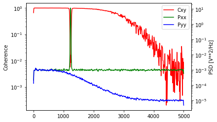
>>>fromscipyimportsignal>>>importmatplotlib.pyplotasplt# Generate two test signals with some common features.>>>fs=10e3>>>N=1e5>>>amp=20>>>freq=1234.0>>>noise_power=0.001*fs/2>>>time=np.arange(N)/fs>>>b,a=signal.butter(2,0.25,'low')>>>x=np.random.normal(scale=np.sqrt(noise_power),size=time.shape)>>>y=signal.lfilter(b,a,x)>>>x+=amp*np.sin(2*np.pi*freq*time)>>>y+=np.random.normal(scale=0.1*np.sqrt(noise_power),size=time.shape)# Compute and plot the coherence.>>>f,Cxy=signal.coherence(x,y,fs,nperseg=1024)>>>f,Pxx=signal.welch(x,fs,nperseg=1024)>>>f,Pyy=signal.welch(y,fs,nperseg=1024)>>>lnxy=plt.semilogy(f,Cxy,color='r',label='Cxy')>>>plt.ylabel('Coherence')>>>plt.twinx()>>>lnx=plt.semilogy(f,Pxx,color='g',label='Pxx')>>>lny=plt.semilogy(f,Pyy,color='b',label='Pyy')>>>plt.ylabel('PSD [V**2/Hz]')>>>plt.xlabel('frequency [Hz]')>>>lns=lnxy+lnx+lny>>>labs=[l.get_label()forlinlns]>>>plt.legend(lns,labs)>>>plt.show()
periodogram (PSD)
Estimate power spectral density using a periodogram.
下面是用 periodogram 计算 PSD 的源码:
defperiodogram(x,fs=1.0,window='boxcar',nfft=None,detrend='constant',return_onesided=True,scaling='density',axis=-1):"""Estimate power spectral density using a periodogram."""x=np.asarray(x)ifx.size==0:returnnp.empty(x.shape),np.empty(x.shape)ifwindowisNone:window='boxcar'ifnfftisNone:nperseg=x.shape[axis]elifnfft==x.shape[axis]:nperseg=nfftelifnfft>x.shape[axis]:nperseg=x.shape[axis]elifnfft<x.shape[axis]:s=[np.s_[:]]*len(x.shape)s[axis]=np.s_[:nfft]x=x[tuple(s)]nperseg=nfftnfft=Nonereturnwelch(x,fs=fs,window=window,nperseg=nperseg,noverlap=0,nfft=nfft,detrend=detrend,return_onesided=return_onesided,scaling=scaling,axis=axis)
例子:
>>>fromscipyimportsignal>>>importmatplotlib.pyplotasplt>>>np.random.seed(1234)# Generate a test signal, a 2 Vrms sine wave at 1234 Hz, corrupted by# 0.001 V**2/Hz of white noise sampled at 10 kHz.>>>fs=10e3>>>N=1e5>>>amp=2*np.sqrt(2)>>>freq=1234.0>>>noise_power=0.001*fs/2>>>time=np.arange(N)/fs>>>x=amp*np.sin(2*np.pi*freq*time)>>>x+=np.random.normal(scale=np.sqrt(noise_power),size=time.shape)# Compute and plot the power spectral density.>>>f,Pxx_den=signal.periodogram(x,fs)>>>plt.semilogy(f,Pxx_den)>>>plt.ylim([1e-7,1e2])>>>plt.xlabel('frequency [Hz]')>>>plt.ylabel('PSD [V**2/Hz]')>>>plt.show()# If we average the last half of the spectral density, to exclude the# peak, we can recover the noise power on the signal.>>>np.mean(Pxx_den[25000:])# 0.00099728892368242854
# Now compute and plot the power spectrum.>>>f,Pxx_spec=signal.periodogram(x,fs,'flattop',scaling='spectrum')>>>plt.figure()>>>plt.semilogy(f,np.sqrt(Pxx_spec))>>>plt.ylim([1e-4,1e1])>>>plt.xlabel('frequency [Hz]')>>>plt.ylabel('Linear spectrum [V RMS]')>>>plt.show()# The peak height in the power spectrum is an estimate of the RMS# amplitude.>>>np.sqrt(Pxx_spec.max())# 2.0077340678640727
spectrogram
Compute a spectrogram with consecutive Fourier transforms.
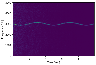
Spectrograms can be used as a way of visualizing the change of a nonstationary signal’s frequency content over time.
源码:
defspectrogram(x,fs=1.0,window=('tukey',.25),nperseg=None,noverlap=None,nfft=None,detrend='constant',return_onesided=True,scaling='density',axis=-1,mode='psd'):"""Compute a spectrogram with consecutive Fourier transforms."""modelist=['psd','complex','magnitude','angle','phase']ifmodenotinmodelist:raiseValueError('unknown value for mode {}, must be one of {}'.format(mode,modelist))# need to set default for nperseg before setting default for noverlap belowwindow,nperseg=_triage_segments(window,nperseg,input_length=x.shape[axis])# Less overlap than welch, so samples are more statisically independentifnoverlapisNone:noverlap=nperseg//8ifmode=='psd':freqs,time,Sxx=_spectral_helper(x,x,fs,window,nperseg,noverlap,nfft,detrend,return_onesided,scaling,axis,mode='psd')else:freqs,time,Sxx=_spectral_helper(x,x,fs,window,nperseg,noverlap,nfft,detrend,return_onesided,scaling,axis,mode='stft')ifmode=='magnitude':Sxx=np.abs(Sxx)elifmodein['angle','phase']:Sxx=np.angle(Sxx)ifmode=='phase':# Sxx has one additional dimension for time stridesifaxis<0:axis-=1Sxx=np.unwrap(Sxx,axis=axis)# mode =='complex' is same as `stft`, doesn't need modificationreturnfreqs,time,Sxx
例子:
>>>fromscipyimportsignal>>>fromscipy.fftimportfftshift>>>importmatplotlib.pyplotasplt# Generate a test signal, a 2 Vrms sine wave whose frequency is slowly# modulated around 3kHz, corrupted by white noise of exponentially# decreasing magnitude sampled at 10 kHz.>>>fs=10e3>>>N=1e5>>>amp=2*np.sqrt(2)>>>noise_power=0.01*fs/2>>>time=np.arange(N)/float(fs)>>>mod=500*np.cos(2*np.pi*0.25*time)>>>carrier=amp*np.sin(2*np.pi*3e3*time+mod)>>>noise=np.random.normal(scale=np.sqrt(noise_power),size=time.shape)>>>noise*=np.exp(-time/5)>>>x=carrier+noise# Compute and plot the spectrogram.>>>f,t,Sxx=signal.spectrogram(x,fs)>>>plt.pcolormesh(t,f,Sxx,shading='gouraud')>>>plt.ylabel('Frequency [Hz]')>>>plt.xlabel('Time [sec]')>>>plt.show()
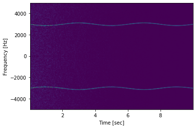
# Note, if using output that is not one sided, then use the following:>>>f,t,Sxx=signal.spectrogram(x,fs,return_onesided=False)>>>plt.pcolormesh(t,fftshift(f),fftshift(Sxx,axes=0),shading='gouraud')>>>plt.ylabel('Frequency [Hz]')>>>plt.xlabel('Time [sec]')>>>plt.show()
istft
Perform the inverse Short Time Fourier transform (iSTFT).
这部分源码比较长,先直接看 stft 的例子,然后是 istft 的例子。
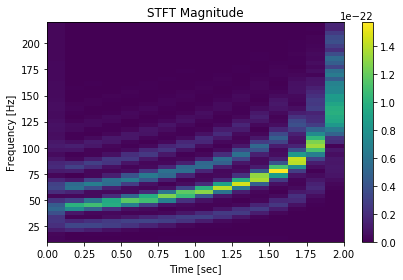
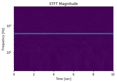
>>>fromscipyimportsignal>>>importmatplotlib.pyplotasplt# Generate a test signal, a 2 Vrms sine wave at 50Hz corrupted by# 0.001 V**2/Hz of white noise sampled at 1024 Hz.>>>fs=1024>>>N=10*fs>>>nperseg=512>>>amp=2*np.sqrt(2)>>>noise_power=0.001*fs/2>>>time=np.arange(N)/float(fs)>>>carrier=amp*np.sin(2*np.pi*50*time)>>>noise=np.random.normal(scale=np.sqrt(noise_power),...size=time.shape)>>>x=carrier+noise# Compute the STFT, and plot its magnitude>>>f,t,Zxx=signal.stft(x,fs=fs,nperseg=nperseg)>>>plt.figure()>>>plt.pcolormesh(t,f,np.abs(Zxx),vmin=0,vmax=amp,shading='gouraud')>>>plt.ylim([f[1],f[-1]])>>>plt.title('STFT Magnitude')>>>plt.ylabel('Frequency [Hz]')>>>plt.xlabel('Time [sec]')>>>plt.yscale('log')>>>plt.show()
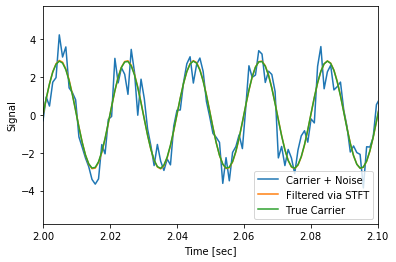
# Zero the components that are 10% or less of the carrier magnitude,# then convert back to a time series via inverse STFT>>>Zxx=np.where(np.abs(Zxx)>=amp/10,Zxx,0)>>>_,xrec=signal.istft(Zxx,fs)# Compare the cleaned signal with the original and true carrier signals.>>>plt.figure()>>>plt.plot(time,x,time,xrec,time,carrier)>>>plt.xlim([2,2.1])>>>plt.xlabel('Time [sec]')>>>plt.ylabel('Signal')>>>plt.legend(['Carrier + Noise','Filtered via STFT','True Carrier'])>>>plt.show()
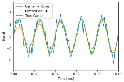
# Note that the cleaned signal does not start as abruptly as the original,# since some of the coefficients of the transient were also removed:>>>plt.figure()>>>plt.plot(time,x,time,xrec,time,carrier)>>>plt.xlim([0,0.1])>>>plt.xlabel('Time [sec]')>>>plt.ylabel('Signal')>>>plt.legend(['Carrier + Noise','Filtered via STFT','True Carrier'])>>>plt.show()
check_COLA
Check whether the Constant OverLap Add (COLA) constraint is met
check_NOLA
Check whether the Nonzero Overlap Add (NOLA) constraint is met
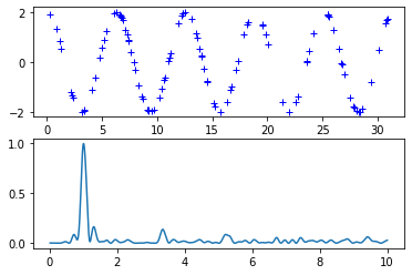
lombscargle
Computes the Lomb-Scargle periodogram.
The Lomb-Scargle periodogram was developed by Lomb 2 and further extended by Scargle 3 to find, and test the significance of weak periodic signals with uneven temporal sampling.
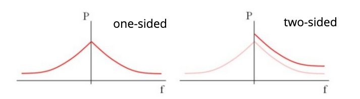
When normalize is False (default) the computed periodogram is unnormalized, it takes the value (A**2) * N/4 for a harmonic signal with amplitude A for sufficiently large N.
When normalize is True the computed periodogram is normalized by the residuals of the data around a constant reference model (at zero).
Input arrays should be 1-D and will be cast to float64.
>>>importmatplotlib.pyplotasplt# First define some input parameters for the signal:>>>A=2.>>>w=1.>>>phi=0.5*np.pi>>>nin=1000>>>nout=100000>>>frac_points=0.9# Fraction of points to select# Randomly select a fraction of an array with timesteps:>>>r=np.random.rand(nin)>>>x=np.linspace(0.01,10*np.pi,nin)>>>x=x[r>=frac_points]# Plot a sine wave for the selected times:>>>y=A*np.sin(w*x+phi)# Define the array of frequencies for which to compute the periodogram:>>>f=np.linspace(0.01,10,nout)# Calculate Lomb-Scargle periodogram:>>>importscipy.signalassignal>>>pgram=signal.lombscargle(x,y,f,normalize=True)# Now make a plot of the input data:>>>plt.subplot(2,1,1)>>>plt.plot(x,y,'b+')# Then plot the normalized periodogram:>>>plt.subplot(2,1,2)>>>plt.plot(f,pgram)>>>plt.show()
fromscipy.signal.windowsimportget_windowdef_triage_segments(window,nperseg,input_length):"""
Parses window and nperseg arguments for spectrogram and _spectral_helper.
This is a helper function, not meant to be called externally.
"""# parse window; if array like, then set nperseg = win.shapeifisinstance(window,str)orisinstance(window,tuple):# if nperseg not specifiedifnpersegisNone:nperseg=256# then change to defaultifnperseg>input_length:warnings.warn('nperseg = {0:d} is greater than input length '' = {1:d}, using nperseg = {1:d}'.format(nperseg,input_length))nperseg=input_lengthwin=get_window(window,nperseg)else:win=np.asarray(window)iflen(win.shape)!=1:raiseValueError('window must be 1-D')ifinput_length<win.shape[-1]:raiseValueError('window is longer than input signal')ifnpersegisNone:nperseg=win.shape[0]elifnpersegisnotNone:ifnperseg!=win.shape[0]:raiseValueError("value specified for nperseg is different"" from length of window")returnwin,nperseg
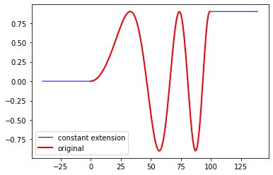
const_ext: Constant extension at the boundaries of an array
Generate a new ndarray that is a constant extension of x along an axis. The extension repeats the values at the first and last element of the axis.
>>>fromscipy.signal._arraytoolsimportconst_ext>>>a=np.array([[1,2,3,4,5],[0,1,4,9,16]])>>>const_ext(a,2)array([[1,1,1,2,3,4,5,5,5],[0,0,0,1,4,9,16,16,16]])# Constant extension continues with the same values as the endpoints of the# array:>>>t=np.linspace(0,1.5,100)>>>a=0.9*np.sin(2*np.pi*t**2)>>>b=const_ext(a,40)>>>importmatplotlib.pyplotasplt>>>plt.plot(np.arange(-40,140),b,'b',lw=1,label='constant extension')>>>plt.plot(np.arange(100),a,'r',lw=2,label='original')>>>plt.legend(loc='best')
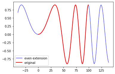
even_ext: Even extension at the boundaries of an array
Generate a new ndarray by making an even extension of x along an axis.
>>>fromscipy.signal._arraytoolsimporteven_ext>>>a=np.array([[1,2,3,4,5],[0,1,4,9,16]])>>>even_ext(a,2)array([[3,2,1,2,3,4,5,4,3],[4,1,0,1,4,9,16,9,4]])# Even extension is a "mirror image" at the boundaries of the original array:>>>t=np.linspace(0,1.5,100)>>>a=0.9*np.sin(2*np.pi*t**2)>>>b=even_ext(a,40)>>>importmatplotlib.pyplotasplt>>>plt.plot(np.arange(-40,140),b,'b',lw=1,label='even extension')>>>plt.plot(np.arange(100),a,'r',lw=2,label='original')>>>plt.legend(loc='best')>>>plt.show()
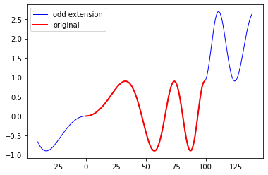
odd_ext: Odd extension at the boundaries of an array
Generate a new ndarray by making an odd extension of x along an axis.
>>>fromscipy.signal._arraytoolsimportodd_ext>>>a=np.array([[1,2,3,4,5],[0,1,4,9,16]])>>>odd_ext(a,2)array([[-1,0,1,2,3,4,5,6,7],[-4,-1,0,1,4,9,16,23,28]])# Odd extension is a "180 degree rotation" at the endpoints of the original array:>>>t=np.linspace(0,1.5,100)>>>a=0.9*np.sin(2*np.pi*t**2)>>>b=odd_ext(a,40)>>>importmatplotlib.pyplotasplt>>>plt.plot(np.arange(-40,140),b,'b',lw=1,label='odd extension')>>>plt.plot(np.arange(100),a,'r',lw=2,label='original')>>>plt.legend(loc='best')>>>plt.show()
zero_ext: Zero padding at the boundaries of an array
Generate a new ndarray that is a zero-padded extension of x along an axis.
fromscipy.signal._arraytoolsimportaxis_slicedefconst_ext(x,n,axis=-1):"""
Constant extension at the boundaries of an array
"""ifn<1:returnxleft_end=axis_slice(x,start=0,stop=1,axis=axis)ones_shape=[1]*x.ndimones_shape[axis]=nones=np.ones(ones_shape,dtype=x.dtype)left_ext=ones*left_endright_end=axis_slice(x,start=-1,axis=axis)right_ext=ones*right_endext=np.concatenate((left_ext,x,right_ext),axis=axis)returnext##########################################################################defeven_ext(x,n,axis=-1):"""
Even extension at the boundaries of an array
"""ifn<1:returnxifn>x.shape[axis]-1:raiseValueError(("The extension length n (%d) is too big. "+"It must not exceed x.shape[axis]-1, which is %d.")%(n,x.shape[axis]-1))left_ext=axis_slice(x,start=n,stop=0,step=-1,axis=axis)right_ext=axis_slice(x,start=-2,stop=-(n+2),step=-1,axis=axis)ext=np.concatenate((left_ext,x,right_ext),axis=axis)returnext##########################################################################defodd_ext(x,n,axis=-1):"""
Odd extension at the boundaries of an array
"""ifn<1:returnxifn>x.shape[axis]-1:raiseValueError(("The extension length n (%d) is too big. "+"It must not exceed x.shape[axis]-1, which is %d.")%(n,x.shape[axis]-1))left_end=axis_slice(x,start=0,stop=1,axis=axis)left_ext=axis_slice(x,start=n,stop=0,step=-1,axis=axis)right_end=axis_slice(x,start=-1,axis=axis)right_ext=axis_slice(x,start=-2,stop=-(n+2),step=-1,axis=axis)ext=np.concatenate((2*left_end-left_ext,x,2*right_end-right_ext),axis=axis)returnext##########################################################################defzero_ext(x,n,axis=-1):"""
Zero padding at the boundaries of an array
"""ifn<1:returnxzeros_shape=list(x.shape)zeros_shape[axis]=nzeros=np.zeros(zeros_shape,dtype=x.dtype)ext=np.concatenate((zeros,x,zeros),axis=axis)returnext
P. Welch, “The use of the fast Fourier transform for the estimation of power spectra: A method based on time averaging over short, modified periodograms”, IEEE Trans. Audio Electroacoust. vol. 15, pp. 70-73, 1967. ↩︎
N.R. Lomb “Least-squares frequency analysis of unequally spaced data”, Astrophysics and Space Science, vol 39, pp. 447-462, 1976 ↩︎
J.D. Scargle “Studies in astronomical time series analysis. II - Statistical aspects of spectral analysis of unevenly spaced data”, The Astrophysical Journal, vol 263, pp. 835-853, 1982
例子: ↩︎
 Credit by Herb